Results
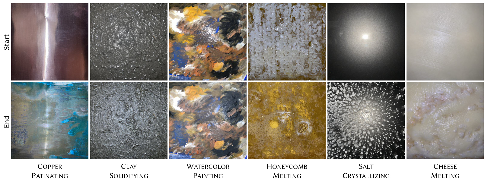
The goal is “exemplar-based time-varying appearance synthesis”.
This interactive gallery shows the input (exemplar) and our results. Please see supplemental for baselines.
Dynamic RGB Texture
Dynamic SVBRDF Map (Relightable)
Abstract
We propose a method to reproduce dynamic appearance textures with space-stationary but time-varying visual statistics. While most previous work decomposes dynamic textures into static appearance and motion, we focus on dynamic appearance that results not from motion but variations of fundamental properties, such as rusting, decaying, melting, and weathering. To this end, we adopt the neural ordinary differential equation (ODE) to learn the underlying dynamics of appearance from a target exemplar.
We simulate the ODE in two phases. At the “warm-up” phase, the ODE diffuses a random noise to an initial state. We then constrain the further evolution of this ODE to replicate the evolution of visual feature statistics in the exemplar during the generation phase. The particular innovation of this work is the neural ODE achieving both denoising and evolution for dynamics synthesis, with a proposed temporal training scheme.
We study both relightable (BRDF) and non-relightable (RGB) appearance models. For both we introduce new pilot datasets, allowing, for the first time, to study such phenomena: For RGB we provide 22 dynamic textures acquired from free online sources; For BRDFs, we further acquire a dataset of 21 flash-lit videos of time-varying materials, enabled by a simple-to-construct setup. Our experiments show that our method consistently yields realistic and coherent results, whereas prior works falter under pronounced temporal appearance variations. A user study confirms our approach is preferred to previous work for such exemplars.
Our Method
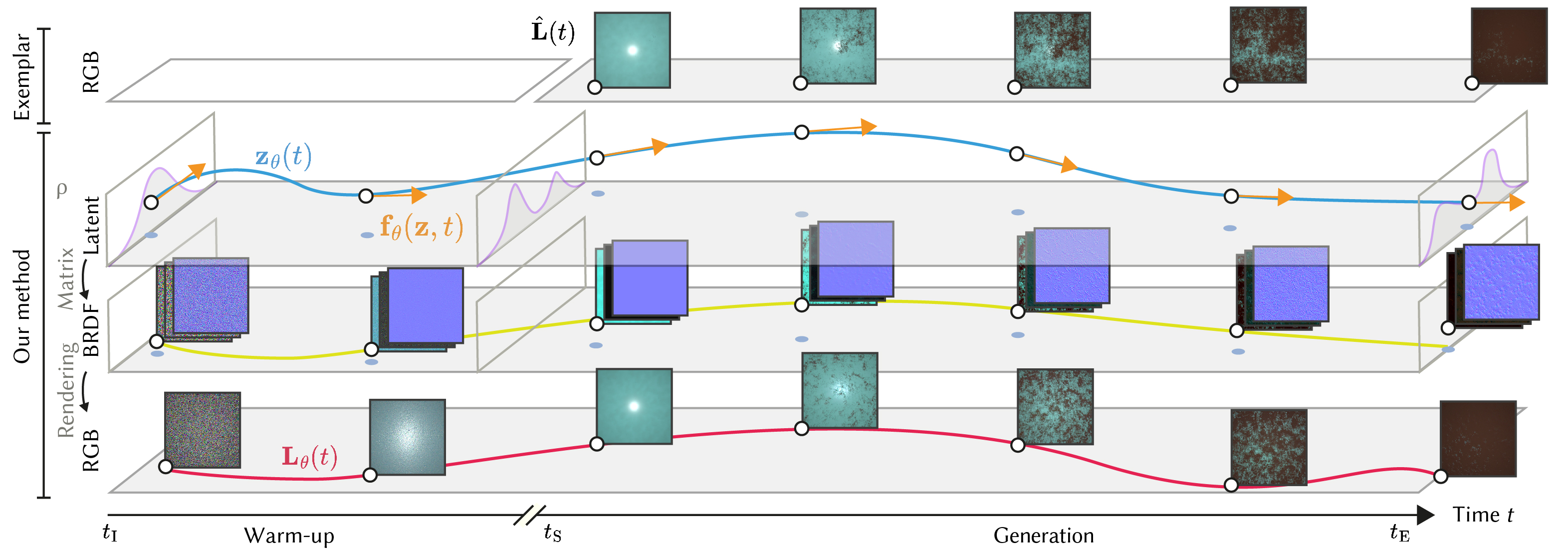
Take a ubiquitous phenomenon, i.e., the rusting of metal, as an example, we all believe that there could be a differential equation describing the chemical interplay between the metal, water, and oxygen over time which eventually produces the rust. But the problem is we don’t know it, or it is just too difficult to write one.
Given the visual observations (top row), we learn the differential equation parameterized by a neural network (orange arrows), directly in a latent space (blue curve), that is, when projected to RGB pixels or combined with a renderer (yellow curve), latents can reproduce the observed dynamics (red curve).

Our Dataset
We capture a pilot dataset for time-varying materials as videos of flash images. We release our data under CC BY 4.0 license – download here.

Presentation Video
Citation
@article{liuNeuralDifferentialAppearance2024,
  title={Neural Differential Appearance Equations},
  author={Liu, Chen and Ritschel, Tobias},
  journal={ACM Transactions on Graphics},
  volume={43},
  number={6},
  pages={1--17},
  year={2024},
  doi={10.1145/3687900},
}
Acknowledgment
Thanks Meta Reality Labs for funding this project. Thanks anonymous reviewers for their insightful suggestions and Michael Fischer for helpful proofreading.
Personally I would like to extend my gratitude to my roommates who allowed me to set up the tiny capture system at home and helped testing, my folks at office who offered me interesting ideas about what materials to capture, and Amber who generously lent me her iPhone 11 and saved the teaser.